5. Lubrication (1D)#
The previous example dealt with the confined fluid close to equilibrium. The flow was induced by small perturbations out of equilibrium to eventually restore the equilibrium state. Now we look at a nonequilibrium case, where the movement of the walls constantly drives the fluid. This situation is commonly found in lubrication. In this tutorial, we’ll look at a journal bearing simulation defined by the following YAML input.
journal_input = """
options:
    output: data/journal
    write_freq: 100
    silent: False
grid:
    dx: 1.e-5
    dy: 1.
    Nx: 100
    Ny: 1
    xE: ['P', 'P', 'P']
    xW: ['P', 'P', 'P']
    yS: ['P', 'P', 'P']
    yN: ['P', 'P', 'P']
geometry:
    type: journal
    CR: 1.e-2
    eps: 0.7
    U: 0.1
    V: 0.
numerics:
    CFL: 0.5
    adaptive: True
    tol: 1e-8
    dt: 1e-10
    max_it: 10_000
properties:
    shear: 0.0794
    bulk: 0.
    EOS: DH
    P0: 101325.
    rho0: 877.7007
    T0: 323.15
    C1: 3.5e12
    C2: 1.23
"""
from GaPFlow import Problem
journal_problem = Problem.from_string(journal_input)
*************************************************************
*                       PROBLEM SETUP                       *
*************************************************************
- options:
  - output                   : data/journal
  - write_freq               : 100
  - use_tstamp               : True
  - silent                   : False
- grid:
  - Nx                       : 100
  - dx                       : 1e-05
  - Lx                       : 0.001
  - Ny                       : 1
  - dy                       : 1.0
  - Ly                       : 1.0
  - dim                      : 1
  - bc_xE_P                  : [True, True, True]
  - bc_xE_D                  : [False, False, False]
  - bc_xE_N                  : [False, False, False]
  - bc_xW_P                  : [True, True, True]
  - bc_xW_D                  : [False, False, False]
  - bc_xW_N                  : [False, False, False]
  - bc_yS_P                  : [True, True, True]
  - bc_yS_D                  : [False, False, False]
  - bc_yS_N                  : [False, False, False]
  - bc_yN_P                  : [True, True, True]
  - bc_yN_D                  : [False, False, False]
  - bc_yN_N                  : [False, False, False]
- geometry:
  - U                        : 0.1
  - V                        : 0.0
  - type                     : journal
  - flip                     : False
  - CR                       : 0.01
  - eps                      : 0.7
- numerics:
  - tol                      : 1e-08
  - max_it                   : 10000
  - dt                       : 1e-10
  - adaptive                 : True
  - CFL                      : 0.5
  - MC_order                 : 1
- properties:
  - shear                    : 0.0794
  - bulk                     : 0.0
  - EOS                      : DH
  - rho0                     : 877.7007
  - P0                       : 101325.0
  - C1                       : 3500000000000.0
  - C2                       : 1.23
  - elastic:
    - enabled                : False
- gp:
- db:
- md:
*************************************************************
*                  PROBLEM SETUP COMPLETED                  *
*************************************************************

     Writing output into: data/2026-05-14_141725_journal
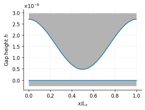
The gap between the shaft and the bearing can be described by a cosine function.
journal_problem.plot_topo()
Before we run the simulation, let us unpack the different sections of the YAML file.
YAML Input#
The options section contains some general options mainly on how and where the simulation output is stored:
options:
    silent: False        # If true, all output to stdout and to files is suppressed, the default is False
    output: data/journal # The name of the simulation output directory, will raise an error if already existent
    use_tstamp: False    # Prepend the simulation output directory with a time stamp (useful to avoid errors due to existent folders)
    write_freq: 1000     # Output frequency (both to stdout and NetCDF file)
The geometry section defines the lubrication problem. It specifies the type of the height profile and the velocities of the walls. Here we look at a journal bearing geometry which can be defined by the nondimensional parameters \(\epsilon\) and \(\mathrm{CR}\):
geometry:
    type: journal # 'bearing' type
    CR: 1.e-2     # clearance ratio
    eps: 0.7      # eccentricity
    U: 0.1        # X velocity of the lower wall
    V: 0.         # Y velocity of the lower wall
The grid section specifies the numerical discretization of the problem and the boundary conditions. For the journal bearing, it makes sense to use periodic boundary conditions.
geometry:
    Lx: 1.e-3           # Length in X
    Ly: 1.              # Length in Y: here 1D so irrelevant
    Nx: 100             # Number of cells in X
    Ny: 1               # Number of cells in Y
    xE: ['P', 'P', 'P'] # BC in x direction (East) for [density, fluxX, fluxY]; 'P' = periodic (other 'D' = Dirichlet, 'N' = Neumann)
    xW: ['P', 'P', 'P'] # BC in x direction (West) for [density, fluxX, fluxY]; 'P' = periodic (other 'D' = Dirichlet, 'N' = Neumann)
    yS: ['P', 'P', 'P'] # BC in y direction (South) for [density, fluxX, fluxY]; 'P' = periodic (other 'D' = Dirichlet, 'N' = Neumann)
    yN: ['P', 'P', 'P'] # BC in y direction (North) for [density, fluxX, fluxY]; 'P' = periodic (other 'D' = Dirichlet, 'N' = Neumann)
Note that 1D simulations like this one should always use periodic BCs in the perpendicular direction (here y). If we wanted to use Dirichlet BCs, we would also need to specify the values to which the boundary cell is fixed, e.g.
    xE_D: 1.
    xW_D: 1.
The time integration settings are defined in the numerics section.
numerics:
    CFL: 0.5        # Courant number used for the adaptive time-stepping
    adaptive: True  # Adaptive time stepping
    tol: 1e-8       # Numerical tolerance for convergence to steady state
    dt: 1e-10       # Time step size (for non-adaptive only)
    max_it: 10_000  # Maximum number of time steps
We have already seen the properties section in previous notebooks. Next to the shear and bulk viscosity, the remaining parameters depend on the type of equation of state used to model the compressible fluid:
properties:
    shear: 0.0794  # Shear viscosity
    bulk: 0.       # Bulk viscosity
    EOS: DH        # Equation of state (here: Dowson-Higginson)
    P0: 101325.    # Reference pressure (for DH-EoS)
    rho0: 877.7007 # Reference density (for DH-EoS)
    T0: 323.15     # Reference temperature (for DH-EoS)
    C1: 3.5e12     # Parameter 1
    C2: 1.23       # Parameter 2
Note that the C1 parameter is four order of magnitude larger than values typically found in the literature. This is intended in order to mimic a (nearly) incompressible fluid with an equation of state as shown in the plot below, where the pressure-density relation is nearly vertical around the reference density.
import numpy as np
import matplotlib.pyplot as plt
from copy import deepcopy
from GaPFlow.models.pressure import eos_pressure

props = {'EOS': 'DH'}
props.update(rho0=877.7007, P0=101325., C1=3.5e8, C2=1.23) # default values
props_comp = deepcopy(props)
props.update(C1=3.5e12)

dens = np.linspace(877.65, 877.75, 300)

fig, ax = plt.subplots(1)

p_comp = eos_pressure(dens, props_comp)
p_incomp = eos_pressure(dens, props)

ax.plot(dens, p_comp,  '-', label='compressible')
ax.plot(dens, p_incomp, '-', label='"incompressible"')

ax.set_yscale('log')
ax.set_xlabel('Density')
ax.set_ylabel('Pressure')
ax.legend();
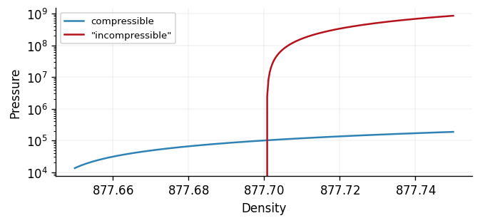
Now we can use the simulation for the nearly incompressible fluids and compare to an analytic solution for incompressible isoviscous fluids and the journal bearing geometry.
Note that the Dowson-Higginson equation of state does not include cavitation, i.e. the possibility of a gas phase. For our model this means that the fluid is assumed to sustain large tensile stresses (negative pressure) without cavitating. Despite not providing physical results in these cases, we use it here because it makes the problem simpler and, more importantly, there exist analytical solutions in literature that we can compare to.
A more realistic behaviour can be obtained with an equation of state that considers cavitation and therefore does not output negative pressures. For that you can use e.g. the Bayada-Chupin equation of state.
journal_problem.run()
-------------------------------------------------------------
Step   Timestep   Time       CFL        Residual
-------------------------------------------------------------
0      3.7972e-11 0.0000e+00 5.0000e-01 1.0000e+00
100    3.7972e-11 3.7972e-09 5.0000e-01 9.6271e-03
200    3.7972e-11 7.5944e-09 5.0000e-01 1.1241e-02
300    3.7972e-11 1.1392e-08 5.0000e-01 2.9111e-03
400    3.7972e-11 1.5189e-08 5.0000e-01 7.5891e-04
500    3.7972e-11 1.8986e-08 5.0000e-01 1.1015e-03
600    3.7972e-11 2.2783e-08 5.0000e-01 8.2644e-04
700    3.7972e-11 2.6581e-08 5.0000e-01 4.1743e-04
800    3.7972e-11 3.0378e-08 5.0000e-01 1.2197e-04
900    3.7972e-11 3.4175e-08 5.0000e-01 1.3118e-05
1000   3.7972e-11 3.7972e-08 5.0000e-01 4.5388e-05
1100   3.7972e-11 4.1769e-08 5.0000e-01 3.6034e-05
1200   3.7972e-11 4.5567e-08 5.0000e-01 1.8486e-05
1300   3.7972e-11 4.9364e-08 5.0000e-01 5.8329e-06
1400   3.7972e-11 5.3161e-08 5.0000e-01 1.8587e-07
1500   3.7972e-11 5.6958e-08 5.0000e-01 1.8239e-06
1600   3.7972e-11 6.0756e-08 5.0000e-01 1.5378e-06
1700   3.7972e-11 6.4553e-08 5.0000e-01 8.2085e-07
1800   3.7972e-11 6.8350e-08 5.0000e-01 2.7721e-07
1900   3.7972e-11 7.2147e-08 5.0000e-01 7.6591e-09
2000   3.7972e-11 7.5944e-08 5.0000e-01 7.2360e-08
2024   3.7972e-11 7.6856e-08 5.0000e-01 2.4640e-09
=================================
Total walltime   : 0:00:07
(265.78 steps/s)
=================================
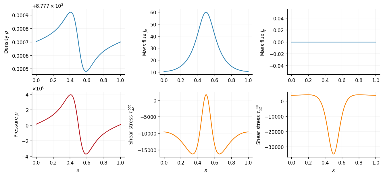
sx, sy = plt.rcParams['figure.figsize']
fig, ax = plt.subplots(2, 3, figsize=(2*sx, 2*sy))
journal_problem.plot(ax=ax)
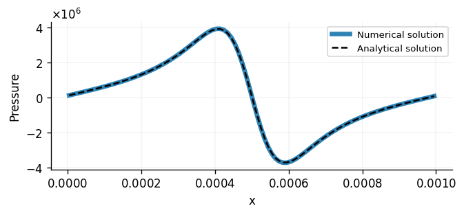
def sommerfeld_solution(x, Lx, mu, U, clearance_ratio, eps, P0):
    """Analytical solution to the journal bearing problem for incompressible fluids.

    Parameters
    ----------
    x : np.ndarray
        Circumferential coordinate
    Lx : float
        Circumference
    mu : float
        Viscosity
    U : float
        Velocity
    clearance_ratio : float
        Clearance ratio
    eps : float
        Eccentricity ratio
    P0 : float
        Boundary pressure

    Returns
    -------
    np.ndarray
        Pressure distribution
    """

    Rb = Lx / (2. * np.pi)
    c = clearance_ratio * Rb
    omega = U / Rb

    prefac = 6. * mu * omega * (Rb / c)**2 * eps

    P = P0 + prefac * np.sin(x / Rb) * (2. + eps * np.cos(x / Rb)) / ((2. + eps**2) * (1. + eps * np.cos(x / Rb))**2)

    return P
p_num = journal_problem.pressure.pressure[1:-1, 1]

Lx = journal_problem.grid['Lx']
U = journal_problem.pressure.geo['U']
CR = journal_problem.pressure.geo['CR']
eps = journal_problem.pressure.geo['eps']
mu = journal_problem.pressure.prop['shear']

Nx = 100
x_ana = np.linspace(0., Lx, Nx + 1)
x_num = (x_ana[1:] + x_ana[:-1]) / 2.

dp = p_num[1] - p_num[0]

p_ana = sommerfeld_solution(x_num,
                            Lx,
                            mu,
                            U,
                            CR,
                            eps,
                            p_num[0] - dp / 2)


fig, ax = plt.subplots(1)

ax.plot(x_num, p_num, lw=4, label='Numerical solution')
ax.plot(x_num, p_ana, '--', color='0.0', label='Analytical solution')

ax.set_xlabel('x')
ax.set_ylabel('Pressure')
ax.legend();