6. Lubrication (2D)#
Two-dimensional problems are configured in the same way but have Ny > 1. Here, we look at the lubricant flow around a model asperity.
asperity_input = """
options:
    output: data/asperity_lj
    write_freq: 100
    use_tstamp: True
grid:
    Lx: 1470.
    Ly: 1470.
    Nx: 100
    Ny: 100
    xE: ['D', 'N', 'N']
    xW: ['D', 'N', 'N']
    yS: ['D', 'N', 'N']
    yN: ['D', 'N', 'N']
    xE_D: 0.8
    xW_D: 0.8
    yS_D: 0.8
    yN_D: 0.8
geometry:
    type: asperity
    hmin: 12.
    hmax: 60.
    U: 0.12
    V: 0.
numerics:
    CFL: 0.5
    adaptive: 1
    tol: 1e-8
    dt: 0.05
    max_it: 5_000
properties:
    shear: 2.15
    bulk: 0.
    EOS: BWR
    T: 1.0
    rho0: 0.8
"""
from GaPFlow import Problem
asperity_problem = Problem.from_string(asperity_input)
*************************************************************
*                       PROBLEM SETUP                       *
*************************************************************
- options:
  - output                   : data/asperity_lj
  - write_freq               : 100
  - use_tstamp               : True
  - silent                   : False
- grid:
  - Nx                       : 100
  - Lx                       : 1470.0
  - dx                       : 14.7
  - Ny                       : 100
  - Ly                       : 1470.0
  - dy                       : 14.7
  - dim                      : 2
  - bc_xE_P                  : [False, False, False]
  - bc_xE_D                  : [True, False, False]
  - bc_xE_N                  : [False, True, True]
  - bc_xW_P                  : [False, False, False]
  - bc_xW_D                  : [True, False, False]
  - bc_xW_N                  : [False, True, True]
  - bc_xE_D_val              : 0.8
  - bc_xW_D_val              : 0.8
  - bc_yS_P                  : [False, False, False]
  - bc_yS_D                  : [True, False, False]
  - bc_yS_N                  : [False, True, True]
  - bc_yN_P                  : [False, False, False]
  - bc_yN_D                  : [True, False, False]
  - bc_yN_N                  : [False, True, True]
  - bc_yS_D_val              : 0.8
  - bc_yN_D_val              : 0.8
- geometry:
  - U                        : 0.12
  - V                        : 0.0
  - type                     : asperity
  - flip                     : False
  - hmin                     : 12.0
  - hmax                     : 60.0
  - num                      : 1
- numerics:
  - tol                      : 1e-08
  - max_it                   : 5000
  - dt                       : 0.05
  - adaptive                 : True
  - CFL                      : 0.5
  - MC_order                 : 1
- properties:
  - shear                    : 2.15
  - bulk                     : 0.0
  - EOS                      : BWR
  - T                        : 1.0
  - gamma                    : 3.0
  - rho0                     : 0.8
  - elastic:
    - enabled                : False
- gp:
- db:
- md:
*************************************************************
*                  PROBLEM SETUP COMPLETED                  *
*************************************************************

   Writing output into: data/2026-05-14_141738_asperity_lj
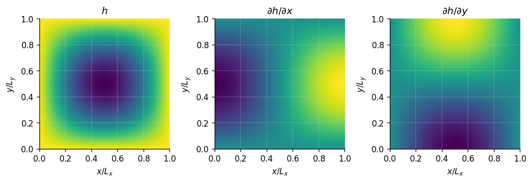
The plot_topo function gives us a qualitative view of the gap topography.
asperity_problem.plot_topo()
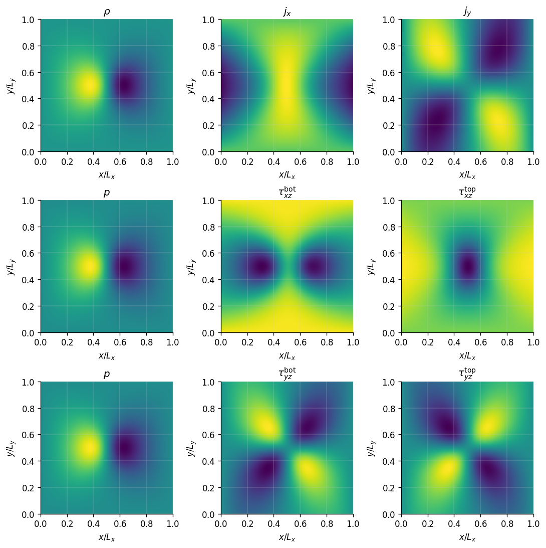
asperity_problem.run()
-------------------------------------------------------------
Step   Timestep   Time       CFL        Residual
-------------------------------------------------------------
0      1.8560e+00 0.0000e+00 5.0000e-01 1.0000e+00
100    1.7522e+00 1.7892e+02 5.0000e-01 1.2871e-03
200    1.7558e+00 3.5422e+02 5.0000e-01 1.5319e-04
300    1.7552e+00 5.2979e+02 5.0000e-01 2.0947e-05
400    1.7553e+00 7.0531e+02 5.0000e-01 2.3957e-06
500    1.7553e+00 8.8084e+02 5.0000e-01 3.0981e-07
600    1.7553e+00 1.0564e+03 5.0000e-01 4.4158e-08
619    1.7553e+00 1.0897e+03 5.0000e-01 2.5133e-09
=================================
Total walltime   : 0:00:18
(34.11 steps/s)
=================================
asperity_problem.plot()