Visualization

GaPFlow provides several command line tools for visualizing simulation output. These tools operate on the output files produced by a simulation run:

• sol.nc: Solution fields (density, momentum, pressure, shear stress)

• topo.nc: Gap height and gradients

• history.csv: Time series of scalar quantities (kinetic energy, residual, etc.)

• gp_zz.csv, gp_xz.csv (optional): GP hyperparameter history

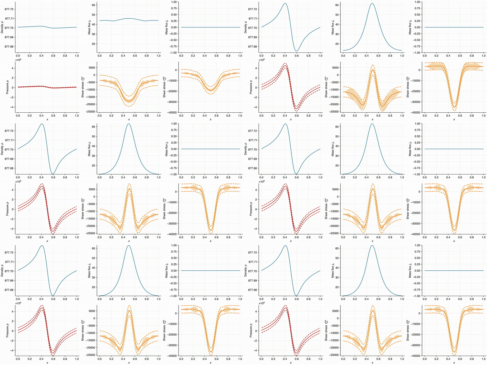
Transient solution of a 1D journal bearing with active learning of the underlying constitutive behavior, created with gpf_animate1d.

File discovery

All visualization commands automatically search for the required output files by recursively walking the directory tree starting from the current working directory. Found simulations are listed with an index and their last-modified date, and you are prompted to select one or more interactively.

For example, running gpf_plot_frame from a directory that contains several simulation output folders might show:

0: data/journal_dh                          20/02/2026 14:30
1: data/journal_dh_gp                       20/02/2026 15:12
Enter keys (space separated or range [start]-[end] or combination of both):

Plotting

gpf_plot_height

Plot the gap height profile from simulation results.

gpf_plot_height [options]

Flag	Type	Default	Description
-d, --dim	int	1	Dimension. 1: plots centerline profile. 2: plots 2D heatmaps of height and gradients.
--show-defo	flag	off	Show displacement in a separate subfigure with the initial gap height as reference.
--show-pressure	flag	off	Show the pressure profile in a separate subfigure.

gpf_plot_history

Plot the time evolution of scalar quantities from history.csv.

gpf_plot_history [options]

Flag	Type	Default	Description
-g, --gp	flag	off	Include Gaussian Process history data (gp_zz.csv and gp_xz.csv).

gpf_plot_frame

Plot a single time step of the solution fields (density, momentum, pressure, shear stress).

gpf_plot_frame [options]

Flag	Type	Default	Description
-d, --dim	int	1	Dimension. 1: line plots. 2: 2D heatmaps.
-f, --frame	int	-1	Frame index to plot. -1 selects the last frame.

gpf_plot_frames

Overlay the centerline solution from all time steps on shared axes. A color gradient indicates time progression (darker = later).

gpf_plot_frames [options]

Flag	Type	Default	Description
-e, --every	int	1	Plot every Nth frame. Useful for reducing clutter when many time steps are available.

Animation

gpf_animate1d

Create an animation of a 1D simulation. Can be displayed interactively or saved to MP4. If GP history files (gp_zz.csv, gp_xz.csv) are present, uncertainty bands are shown automatically.

gpf_animate1d [options]

Flag	Type	Default	Description
-s, --save	flag	off	Save animation to an MP4 file.
-p, --path	str	.	Path to search for simulation output files.
-m, --mode	str	single	File selection mode (single: interactive selection of one simulation).

gpf_animate2d

Create an animation of a 2D simulation as a grid of heatmaps evolving over time.

gpf_animate2d

This command has no additional arguments.